Faster, Simpler Method Scaling Across Particle Sizes Using the Waters Columns Calculator Compared to Manual Calculation Workflow

When scaling an established analytical method across columns packed with different particle sizes and different column configurations (internal diameters and lengths), the amount of time that is required outside of the lab to produce the equivalent method conditions is considerable. When dealing with a gradient method, the calculations required include determining the new flow rate, gradient times, and injection volume. An analyst can perform these calculations manually using the appropriate equations or tools like the Waters Columns Calculator. This application brief examines two scaling workflows by first performing a theoretical scale-down experiment manually using the appropriate method scaling equations, and then repeating the experiment using the scaled-down conditions generated by the Waters Columns Calculator. Strong agreement between manual calculations and the results using the Waters Columns Calculator validate the Waters Column Calculator for its use in scaling methods effectively, with a significant improvement in time savings and a reduction in potential calculation errors and/or uncertainties.

Benefits

• Scale methods fast with minimal user input using the Waters Columns Calculator
• Automatically calculate needed values for new methods
• Guidance on system dwell volume needs provided based on inputs

Scaling a reversed-phase liquid chromatography (RPLC) method between particle sizes is done for a variety of reasons. Scaling-up to columns that have larger particle sizes is often performed when moving a method that was generated using a high throughput column (sub ~2 µm particles) to a column that is more likely used in a routine Quality Control (QC) environment or in the beginning steps of preparatory LC workflows (>3 µm particles). Method development processes often use sub-2 µm particles to maximize separation speed, taking advantage of the increased efficiency these smaller particles produce. However, these smaller particle columns are not always used in a QC environment. Robustness and reproducibility are paramount in QC environments and using sub-2 µm particles can present a challenge, as these columns require instrumentation that can operate at higher operating pressures and columns packed with sub-2 µm particles can often clog from sample excipients or endogenous compounds if proper sample cleanup is not performed. Scaling methods down to columns that use smaller particle sizes, from 5 µm to <5 µm, are routinely performed. An example of this can be found with liquid chromatograph methods within United States Pharmacopeia (USP) monographs, which are often scaled to columns that contain smaller particle sizes to provide the benefits of reduce sample runtime and reduce solvent usage and cost. 1–4 It should be noted that scaling methods to preparatory scale requires different calculations than shown here. Preparatory workflows have a different focus than analytical scale workflows and should therefore be treated separately.

This application brief examines the workflow of performing a scaling experiment. A theoretical method will be examined using 5 µm particles which will be scaled down to 2.5 µm particle column to simulate modernization of an existing method. This will be done using two distinct workflows. First, the scaling calculations will be performed manually, using the equations specified in the USP General Chapter <621>. Next the same method will be scaled using the Waters Column Calculator, and the resulting values will be compared to the manual results.

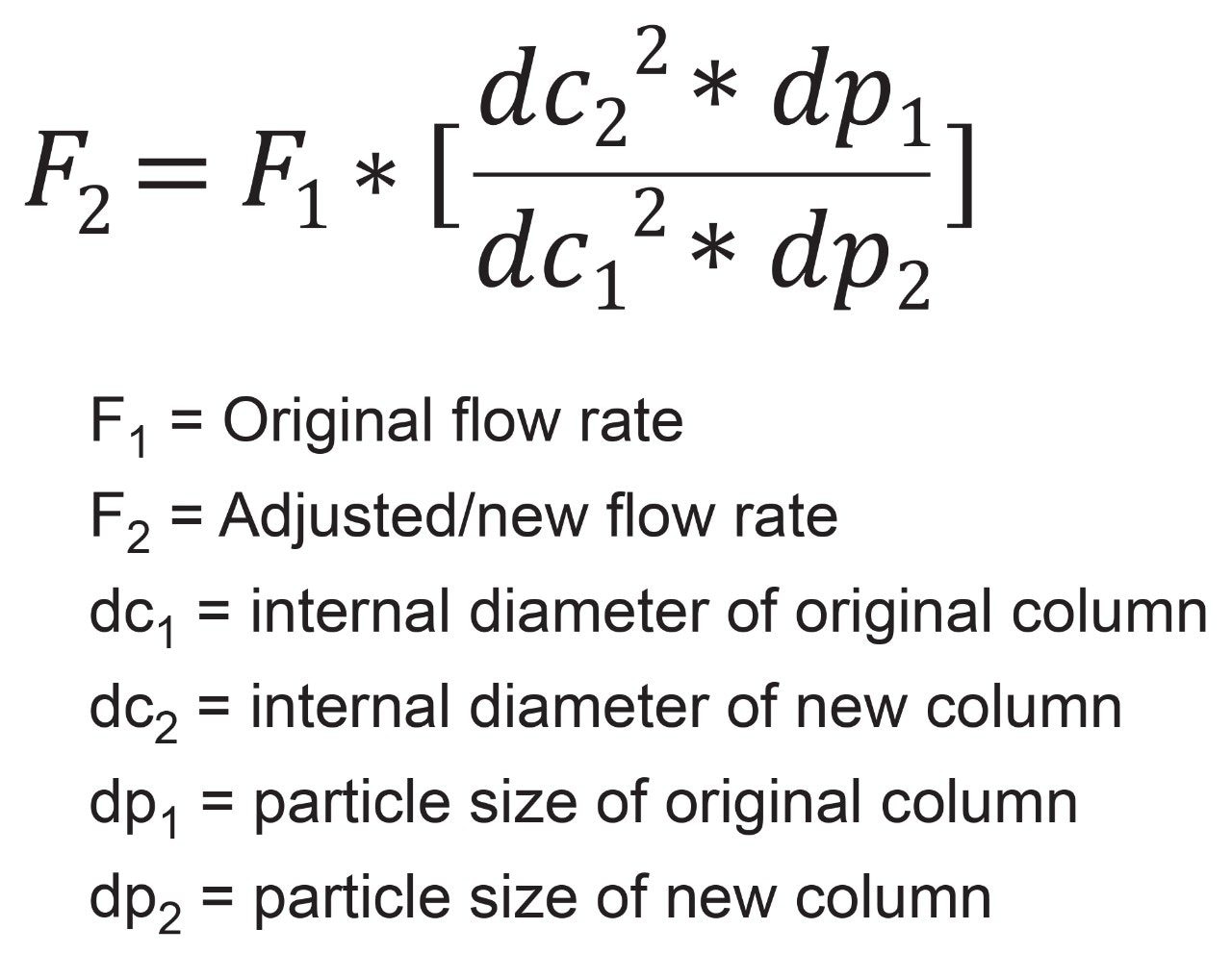
USP General Chapter <621> outlines the needed calculations to properly scale a method between columns of different particle sizes and dimensions. Additional requirements are set for validated methods and must be observed, however for this application brief, no such requirements will be in effect. To properly scale a method, whether it be to scale-up or scale-down, the first calculation required is the new flow rate. All subsequent calculations, except for injection volume, will require the flow rate of the new column. Equation 1 shows the calculation for new flow rate, where F₂ is the new flow rate, F_­1­ is the original flow rate, dc_x is the internal diameter of the column and dp_x is the particle size of the column. In this case, any variables with a subscript of 1 will be associated with the original method conditions, and anything with a subscript 2 will be the new conditions.

The above equation takes into consideration the internal diameter and particle size of both columns to ensure that the correct linear velocity is applied to both. By matching linear velocity on both columns, the analytes being tested will have equal time to interact with the stationary phases and should produce comparable results.

For this application brief, the organic impurities assay of the pharmaceutical drug risperidone will be scaled. As outlined in the USP monograph, the original flow rate is set to 2 mL/min, with a 4.6 x 250 mm, 5 µm column.⁵ The new column will be a 3.0 x 100 mm packed with 2.5 µm particles. Plugging in the values and calculating for the new flow rate indicates a flow rate of 1.70 mL/min should be used, Figure 1. 

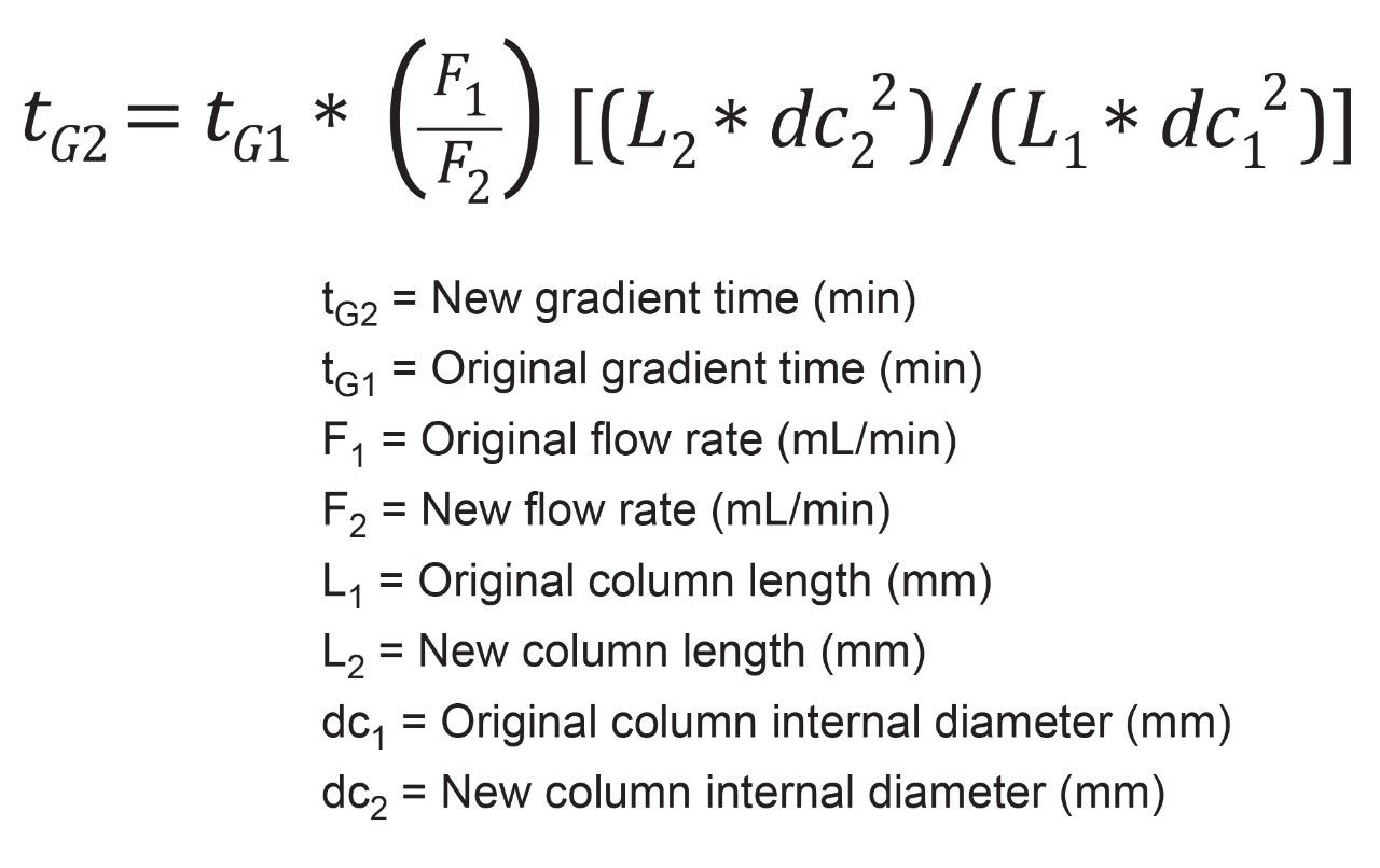
Once a new flow rate is determined, the next step is calculating the new runtime, also called gradient time. This calculation can be used for both gradient and isocratic analyses, however, gradient tests require additional calculations, particularly the gradient ratio. USP <621> outlines the following equation to calculate new gradient time, t_G2.⁶ For this equation, as before, any variable with subscript 1 relates to the original testing conditions, while those with subscript 2 are for the new conditions. The variable t_Gx indicates gradient time, F_x indicates flow rate, L_x column length, and dc_x internal diameter of the column.

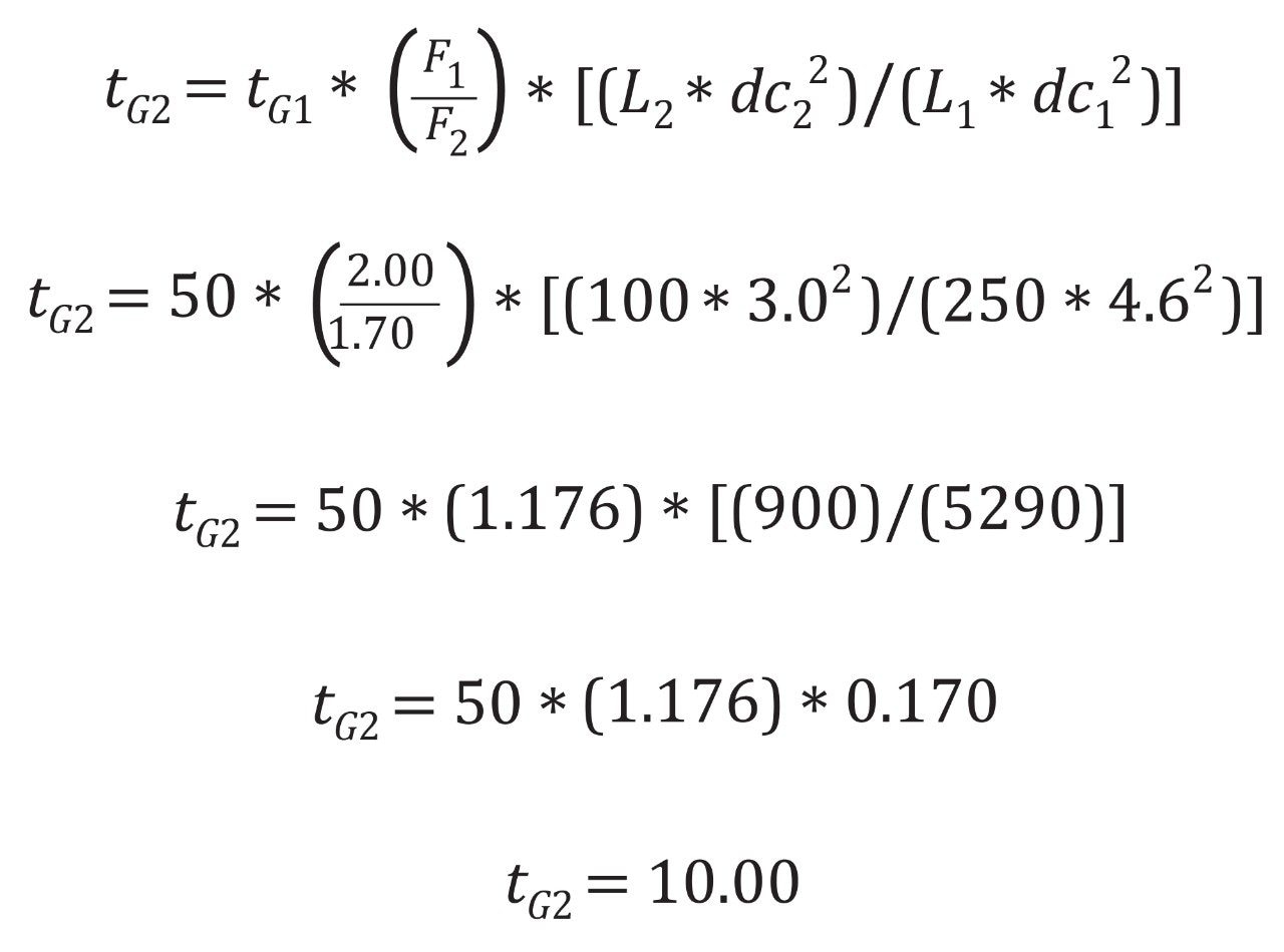
Plugging in the values from the organic impurities of the risperidone assay and solving for t_G2, results in the new gradient time of ten minutes, Figure 2. With an original time of analysis of 50 minutes, and an updated time of ten minutes, a five times decrease in runtime can be achieved by scaling down this method, translating to increased sample throughput.

For isocratic analyses, the final calculation required is injection volume. However, for gradient methods, additional steps are needed before calculating injection volume, which include the determination of the gradient time ratio and applying that ratio to the original gradient table to produce the new gradient table. The gradient time ratio is simple to calculate using the t_G2 and t_G1 values from earlier. In this case, the gradient ratio would be 10/50 or 0.2. This ratio can then be applied to each step in the gradient table as shown in table 1.

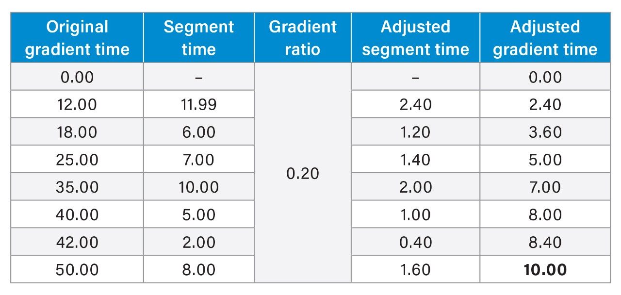
For each step of the gradient, the segment time must be calculated. Examining Table 1, lines one and two, the first segment time is 12.00, as that is the time difference in time between the first step and second step. It is critical to use segment time for adjustments instead of gradient time as the ratio is only applicable to the individual segments or “steps” of the gradient. Examining the adjusted segment time and adjusted gradient time, we see that the adjusted gradient time is the sum of the previous line adjusted gradient time and the adjusted segment time. The last step of the gradient should have an adjusted gradient time that matches the t_G2 value calculated earlier, such as the case here.

Now that the new gradient table, gradient time, and flow rate have been determined, the new injection volume can be calculated. This step is independent of earlier calculations and can be performed when desired. Equation 3 shows how to adjust injection volume based on original injection volume, V_inj1, column length, L_x, and column internal diameter dc_x. As with previous equations, any variable with a subscript 1 is associated with original conditions, while subscript 2 is the adjusted conditions.

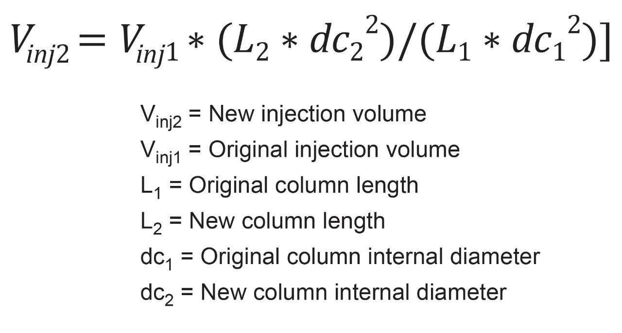
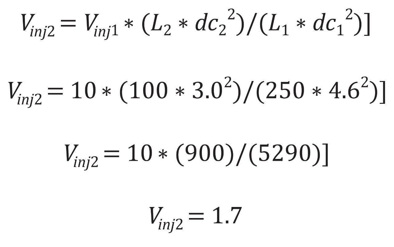
In the original test conditions, a 10 µL injection is executed on a 4.6 x 250 mm column. As discussed previously, the new column is a 3.0 x 100 mm. Figure 3 shows the calculation for the new injection volume.

With all the calculations finished, an analyst could now go and run the new column using the new conditions outlined to determine if comparable chromatographic results are achieved. Performing these calculations manually takes considerable time and effort, especially for complex gradient methods where the gradient table also needs to be adjusted. Additionally, manual calculation of these parameters introduces potential for human error and any slight miscalculation can lead to drastic differences in the results, and ultimately testing conditions. Simplifying the workflow for scaling methods can not only reduce the time needed to perform these calculations, but also reduce the potential for human error. The easiest and most straightforward way to simplify this workflow is to use a calculator. The Waters Column Calculator is a free software that calculates new method conditions based on the input of critical pieces of information, like column dimensions, particle size, flow rate, and gradient profile. Using the example from before, these values were input into the column calculator to scale the method from a 4.6 x 250 mm, 5 µm column to a 3.0 x 100 mm, 2.5 µm column. Figure 4 shows the column calculator and the results of the scaling experiment.

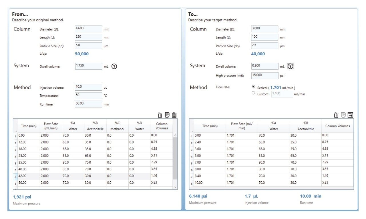
Using the Waters Columns Calculator is considerably easier than the manual calculation of new testing conditions. On the left side of the tool, simply input original column dimensions, particle size, injection volume, column temperature, and runtime. For gradient methods, the gradient table on the left-hand side must also be filled in with the information from the original test conditions. System dwell must also be included, especially for gradient methods, as dwell can have a considerable impact on performance. Unlike manual calculations, including system dwell measurements in the Waters Columns Calculator will allow the calculator to determine if any additional steps are needed for scaling the method due to differences in system dwell. Manual calculations do not include any formulas for this. System dwell is easily measured using a simple protocol.⁷

Next, the user needs to input their new column dimensions on the right-hand side. If a gradient method is being scaled, and the system is also being changed, the new system dwell volume must also be included. In the example shown here, the system is changing from an HPLC to a UPLC, and the systems’ dwell volumes are included in the tool. For this example, no extra steps are needed due to dwell, however should those steps be needed, the calculator would show them in the bottom right corner, next to runtime.

Once those pieces of information are input, the calculator will perform all the calculations needed in real time. As shown on the right-hand side, the calculator is indicating that the new flow rate of the method is 1.701 mL/min, with a total runtime of ten minutes. Additionally, a 1.7 µL injection is needed for the new testing conditions. All three of these values agree with the manual calculations performed earlier. Further agreement can be seen when examining the new gradient table on the right-hand side, which matches the values for the gradient table that were manually determined.

Given that both approaches to scaling the method produce the same results, the true benefit is in the time savings and reduction of the possibility for error. Using the Waters Columns Calculator eliminates doubt in the calculations and allows an analyst to scale a method and get back to running samples more quickly.

Scaling an analytical method in RPLC can require a fair amount of pre-work to ensure the new conditions will provide similar chromatographic results as the original conditions. This pre-work includes calculating various parameters including injection volume, flow rate, and runtime. For gradient methods, the gradient table also needs to be adjusted to ensure the slope of the gradient and each segment of the gradient is equivalent. These calculations, outlined in USP <621>, are complex and take some time and effort to work through. The manual calculation of these values can introduce human error, leading to the wrong conditions being tested, wasting both time and money.

The Waters Column Calculator is a free tool to perform these calculations with minimal user input, reducing the potential for human error and greatly increasing the speed at which these calculations can be performed. An analyst simply needs to input certain critical values like column dimensions and original test conditions, and the calculator determines the new flow rates, runtimes, and gradient tables. The Waters Columns Calculator is a versatile tool that works for both scaling up and scaling down experiments. To illustrate this, a single method was scaled both manually and with the Waters Columns Calculator.

1. Berthelette K, Turner JE, Walter TH, Haynes K. Modernization of the Acetaminophen USP Monograph Gradient HPLC for Impurities Using USP <621> Guidelines and MaxPeak Premier HPS Technology. Waters application note. 720007846, Accessed 27-Feb-2023.
2. Berthelette K, Nguyen JM, Turner JE, Savage D. Reductions in Cost and Time by Modernizing a USP Monograph from HPLC to UHPLC to UPLC Instrumentation and Columns. Waters Application note. 720007427, Accessed 27-Feb-2023.
3. Dlugasch AB, Simeone J, McConville PR. Scaling a USP Gradient Method on the ACQUITY Arc System in Support of Lifecycle Management. Waters Application note. 720006620, Accessed 27-Feb-2023.
4. Sehajpal J, Fairchild JN, Swann T. USP Method Modernization for Lidocaine Formulations using XBridge Columns and Different LC Systems. Waters Application note. 720006179, Accessed 27-Feb-2023. 
5. Risperidone USP monograph. Accessed 20-Feb-2023. https://online.uspnf.com/uspnf/document/1_GUID-46A907B2-576F-4C97-8BA1-6C17E8249978_4_en-US?source=Activity
6. USP General chapter <621>. Accessed 20-Feb-2023. https://online.uspnf.com/uspnf/document/1_GUID-6C3DF8B8-D12E-4253-A0E7-6855670CDB7B_6_en-US?source=TOC
7. How do I determine system dwell volume – WKB50707. Waters Knowledge Base article. Accessed 27-Feb-2023. https://support.waters.com/KB_Chem/Other/WKB50707_How_do_I_determine_system_dwell_volume